Let’s start with MNIST

So, lots of Coursera subjects done and then crap all produced. Geoffrey Hinton’s Neural Networks for Machine Learning was very interesting. I’ll do something with that.

Interesting paper number one: “Stacked Denoising Autoencoders: Learning Useful Representations in a Deep Network with a Local Denoising Criterion” by Pascal Vincent, Hugo Larochelle, Isabelle Lajoie, Yoshua Bengio and Pierre-Antoine Manzagol. Stacked = stacked. Denoising = get rid of noise. Autoencoders = things (single-hidden layer neural networks in this case) that encode themselves (not true here, they encode the input, and they try to make their output look like their input). They trained these stacked denoising autoencoders (SDAs) on a few standard datasets and use the hidden layer representations as inputs to support vector machines (SVMs) for classification. They get very good results.

I want to replicate these results to see how much fidgeting would need to be done to get such good results and to try to gauge how easy it would be to use the same technique for other problems. I can also document the parameters that weren’t specified in the paper.

The easiest dataset they used for me is MNIST, which is an (over)used collection of 70000 images of hand-written single-digit numbers (from 0 to 9) created by Corinna Cortes and Yann LeCun.  You can get it from http://yann.lecun.com/exdb/mnist/ or preprocessed so that all pixel intensity values are scaled to the range 0 to 1 and in a more semi-standard format from the libsvm dataset page (which is what I did).

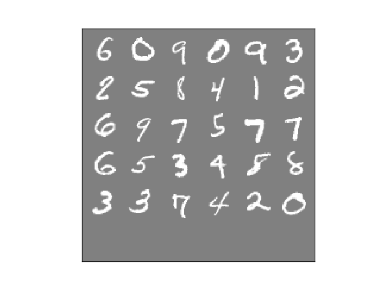
The images are all grayscale 28×28 images (processed from 20×20 black and white images) with the number centered in the image and spanning most of it. The numbers were collected from real people (government employees and high-school students), and they look like normal hand-written digits in all the usual fucked up ways that people write numbers.  eg here’s a sample my computer picked at random:

The problem is known to be easy. The paper uses SVMs with Gaussian radial basis function (RBF) kernels as the baseline to compare against, and they get 98.6% right.  SVMs = black magic classifiers. How I understand them: they work by mapping all the data to higher dimensions and then drawing a hyperplane (ie a line/plane in n-1 dimensions) between the samples to divide them as well as possible (which is pretty much how I think of most classifiers). The kernels they use are functions of the dot product of the samples. I think of them as the way to measure the distances between samples and I thought they could also be interpreted as how the mapping to higher dimensions is done but I read Someone Smart saying this wasn’t the case, so it most likely isn’t (I can’t remember who or where that was, but it seemed authoritative enough to stick).

The most popular SVM package seems to be libsvm by Chih-Chung Chang and Chih-Jen Lin. It has nice command-line tools, python bindings and nice utils (also written in python) so I was sold.

There are two important hyperparameters to tweak with SVMs that use gaussian RBFs. First one is the cost (C) of misclassification (ie where to set the trade off between making the dividing hyperplane more complicated versus how much we want the plane to divide the training dataset exactly). Second one is gamma (g), which is how tight we want the Gaussian RBFs to be (g is inversely proportional to the standard deviation of those gaussians).

SVMs only classify between two classes, and there are a lot of different ways to extend that to multiclass classification (like picking from 0 to 9). One way is to build one classifier per target classification (10 in this case). When you train each classifier, you put the target class samples on one side, and all other samples on the other side (eg when training the classifier for the digit 3, you call all the samples of 3s true, and all the samples of non-3s (0s, 1s, 2s, 4s, 5s, 6s, 7s, 8s and 9s) false) . When you are testing, you see which of the classifiers says it is most likely that that target class is true.  This is called one vs all classification.

Another “simple” way to do multiclass classification, and the way that libsvm does it by default, is to build a classifier for each pair of target classes (eg one for the 1s vs the 2s, one for the 7s vs the 8s, one for the 1s vs the 7s, etc). n * (n-1) / 2 classifiers in total (45 in this case).  Then when you test a sample you run the sample on all n * (n-1) / 2 classifiers and keep a tally of which class wins most of the contests for that sample, and claim the winner as the class of the sample. This is one of the one vs one classification systems. Intuitively to me the one vs all system seems better, but libsvm and others seem to like the one vs one and claim it works better. There are many other ways of mapping binary classification to multiclass classification, and I’ll probably try some in the future.

libsvm comes with a little util called grid.py that looks for the best hyperparameters by sampling the two hyperparameters on a log/log grid, training and doing cross-validation on the data you give it.  The MNIST data is split into 60000 training samples and 10000 test samples. I picked 6000 out of the 60000 training samples to do the grid search to speed the process up.  Running grid.py with default parameters samples 110 points on the grid and took about 36 hours on my i7-870 on those 6000 samples (this was before I discovered libsvm-cuda, but I’ll write about libsvm-cuda later).

While grid.py was running I noticed that the gamma parameter was very important and the cost was completely uninteresting as long as it was sufficiently high (anything bigger than 2). grid.py came back with log2 gamma = -5 (0.03125) and cost = some number but I picked 64. I probably should have done some more fine-grained searching on the gamma parameter but I thought 36 hours was enough runtime for my computer

Training with those parameters on the whole learning set, and testing on the testing set gives me 98.57% right. Which is ridiculous. Practically no preprocessing, only scaling between 0 and 1, no coding and automated tweaking, and it gets almost all numbers right. SVMs are something I’m going to have to keep trying on other datasets.

No coding is required for the above.  Assuming you have libsvm compiled and you have, say, the libsvm source directory under “libsvm”, the full list of commands to get the above results would be:

# subselect 6000 training samples to run the grid faster
libsvm/tools/subset.py mnist.scale 6000 mnist6000.scale 
# grid to find the best hyperparameters
libsvm/tools/grid.py mnist6000.scale
# wait for a long time and read output from grid.py giving you the best hyperparameters
# use them to train a model
svm-train -c 64 -g 0.03125 mnist.scale mnist.model
# see how well that did
svm-predict mnist.scale.t mnist.model mnist.outputguesses

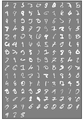
By the way, here are the 143 cases that it got wrong:

That’s the straight SVM result replicated. Next to replicate the interesting bit of the autoencoder prepocessing.